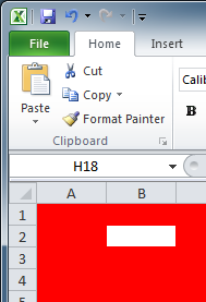
If you’ve ever worked on a complicated Excel spreadsheet you’ve probably ended up with protected (locked) cells everywhere and eventually lost track of which are protected and which aren’t.
Here’s a quick was to detect and view the protected cells in your spreadsheet.
Please note: by default all cells in a spreadsheet are locked – if you haven’t unlocked any cells this process will correctly display everything as locked.
- Open your spreadsheet.
- If the spreadsheet is currently protected you will need to turn this off in the ‘Review’ tab
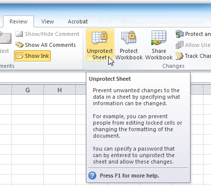
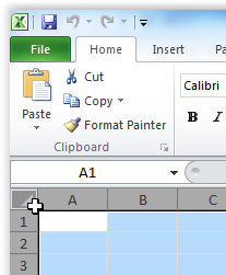
- Now you need to select all cells, this can be done by pressing Ctrl and A on your keyboard or using the select all cells icon which is between the A and 1
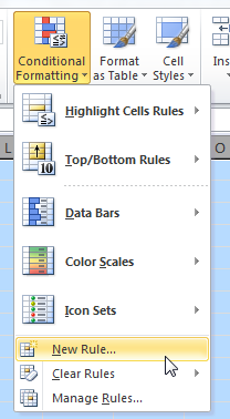
- Now on the ‘Home’ ribbon menu click on ‘Conditional Formatting’ and select ‘New Rule’
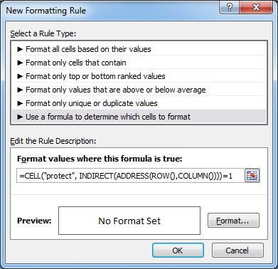
- From the list select ‘Use a formula to determine which cells to format’
- Under ‘Format values where this formula is true’ enter the following
-
=CELL("protect", INDIRECT(ADDRESS(ROW(),COLUMN())))=1 - Click on the ‘Format’ button
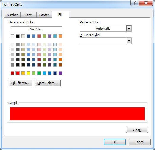
- Click on the ‘Fill’ tab
- Select the colour which will display for locked cells – e.g. red
- Click ‘OK’ and ‘OK’ again to save the changes
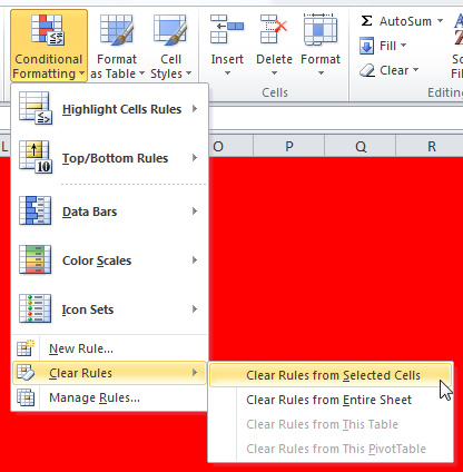
- To return the fields to their normal background click on the ‘Conditional Formatting’ button and then select ‘Clear Rules’ -> ‘Clear Rules from Entire Sheet’
Reference: http://a32.me/2010/04/excel-locked-unlocked-cells/
