Excel can help manage team rosters, including automating two-weekly rotations.
On this pageJump to a section
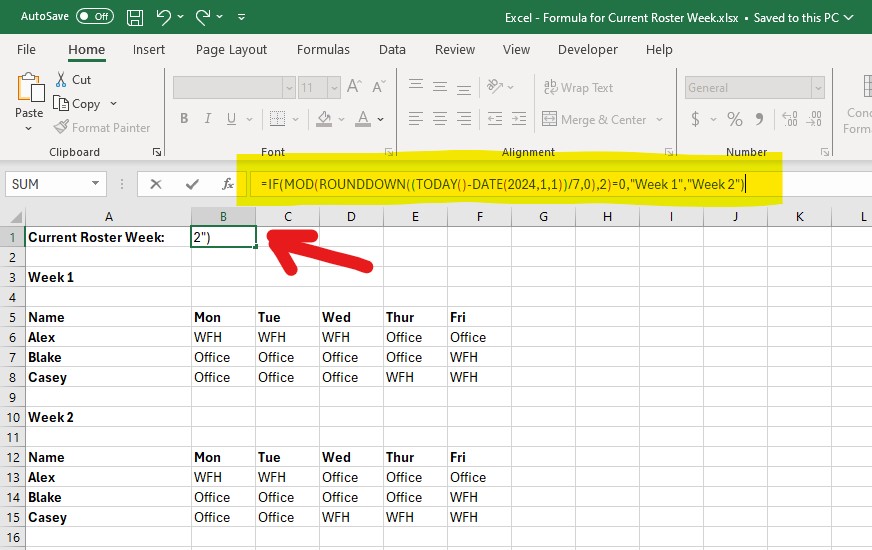
This guide shows how to use a formula in Microsoft Excel to automatically display the current roster week, alternating between “Week 1” and “Week 2”.
For this example, assume that Week 1 started on 1 January 2024, and each week begins on a Monday.
Example Team Roster
Current Roster Week: Current Roster Week – Week 1 or Week 2
Week 1
| Name | Mon | Tue | Wed | Thur | Fri |
|---|---|---|---|---|---|
| Alex | WFH | WFH | WFH | Office | Office |
| Blake | Office | Office | Office | Office | WFH |
| Casey | Office | Office | Office | WFH | WFH |
Week 2
| Name | Mon | Tue | Wed | Thur | Fri |
|---|---|---|---|---|---|
| Alex | WFH | WFH | Office | Office | Office |
| Blake | Office | Office | Office | Office | WFH |
| Casey | Office | Office | WFH | WFH | WFH |
Steps
-
Open Excel File
Open the Excel file where you want to track the roster week. -
Create a Cell for the Current Roster Week
Choose a cell (e.g., E1) where the current roster week will be displayed. -
Enter the Formula
In the chosen cell, enter:="Current Roster Week: " & IF(MOD(WEEKNUM(TODAY(), 2), 2)=0, "Week 2", "Week 1")
-
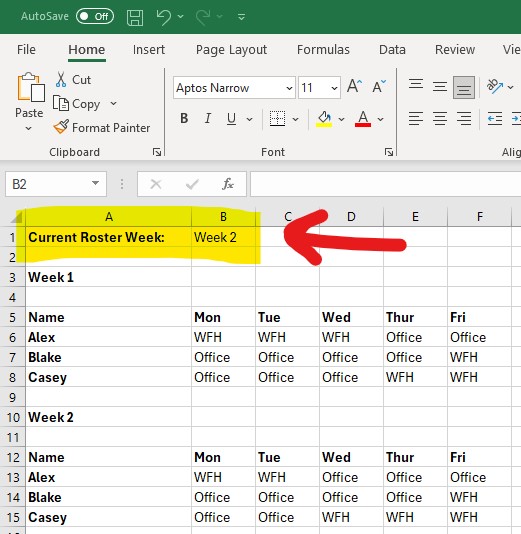
Apply and Verify
Press Enter. The cell will show either “Current Roster Week: Week 1” or “Current Roster Week: Week 2”, depending on the current date.
How does the formula work?
- TODAY(): Returns today’s date.
- WEEKNUM(TODAY(), 2): Finds the current week number of the year, assuming Monday as the first day of the week.
- MOD(…, 2): Checks whether the week number is even or odd.
- Even week number ⇒ “Week 2”
- Odd week number ⇒ “Week 1”
- IF(…): Chooses “Week 1” or “Week 2” based on the result of MOD.